Subjective Bayesian Priors in mogp
Our R interface to mogp allows users to specify their own subjective priors for the parameters of each of the emulators they are fitting simultaneously and in an intuitive way. However, you are able to do this directly with mogp, so why use our package at all?
The reason is that, absent specific knowledge about the output(s) you
are emulating, most users just want default choices that fit well, with
perhaps a little flexibility (say to indicate that one parameter really
should be active and another shouldn’t). The most common approach is to
fit the hyperparameters by maximum likelihood. This is the approach of
the widely used dicekriging package, and the default approach for
mogp_emulator. However, maximum likelihood approaches are not
generally appropriate for building emulators, because there is a ridge
on the likelihood surface.
There are 2 potential issues. The first is the confounding between σ2, the regression line and the correlation parameters. So, a regression line close to the least squares estimate, a low σ2 and a moderate correlation is the solution you would like, but if σ2 is made large and the correlation made large, good interpolators (on the ridge of the likelihood surface) are found whatever line is fit. You can often see this when fitting constant mean functions, when the fit has a mean parameter that is a long way from the data. The second is that, whatever the model you are trying to emulate, it is normally the case that a weakly stationary Gaussian process is not “generative”, and so the “best” fits to the data (in terms of the likelihood function) are those with a large variance (often in the nugget) and with low correlation. An example of the motivating problem is given below.
Preliminaries
We start by specifying the directory where mogp_emulator is installed
so that the python is correctly imported. Please note that your
directory will be different from mine.
mogp_dir <- "~/Dropbox/BayesExeter/mogp_emulator"
setwd('..')
source('BuildEmulator/BuildEmulator.R')
The ridge on the GP likelihood surface
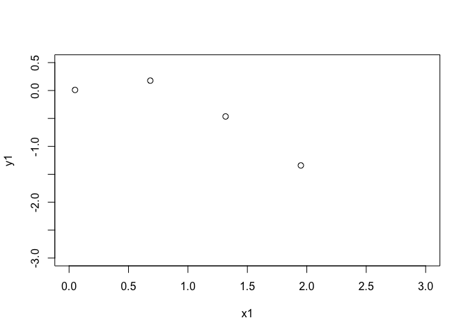
First make a simple function to emulate in 1D so we can see what is happening.
n_train <- 4
x_scale <- 2
x1 <- seq(from=0.05,to=1.95,length.out = n_train)
y1 <- sqrt(x1)*sin(x1 - x1**2)
x <- data.frame(x1, y1)
plot(x1,y1,xlim=c(0,3),ylim=c(-3,0.5),cex=1.1)
xpreds <- seq(from=0,to=3,length.out = 100)
Now build an emulator with a linear mean function and some weakly
informative priors to ensure we get a good fit (this should create the
type of emulator we want automatically and we spend most of this
vignette discussing these prior choices). The nugget is fit adaptively
inside mogp_emulator so is set to be as small as possible to get the
numerics to work.
target_list <- extract_targets(x, target_cols = c("y1"))
inputs <- target_list[[1]]
targets <- target_list[[2]]
inputdict <- target_list[[3]]
mean_func <- "y1 ~ x1"
priors <- list(mogp_priors$NormalPrior(0, 10.),
               mogp_priors$NormalPrior(0, 10),
               mogp_priors$NormalPrior(0., 0.125),
               mogp_priors$InvGammaPrior(2., 1.))
gp <- mogp_emulator$GaussianProcess(inputs, targets,
                                    mean=mean_func,
                                    priors=priors,
                                    nugget="adaptive",
                                    inputdict=inputdict)
p <- mogp_emulator$fit_GP_MAP(gp)
plot(x1,y1,xlim=c(0,3),ylim=c(-3,0.5),cex=1.1)
tpreds <- gp$predict(xpreds,deriv = FALSE)
points(xpreds,tpreds$mean,col=4,type='l')
points(xpreds, tpreds$mean + 2*(sqrt(tpreds$unc)),col=4,type="l",lty=2)
points(xpreds, tpreds$mean - 2*(sqrt(tpreds$unc)),col=4,type="l",lty=2)
p$theta
## [1] -0.37761909 -0.39385298 0.02827789 -0.97248789 -0.22036307
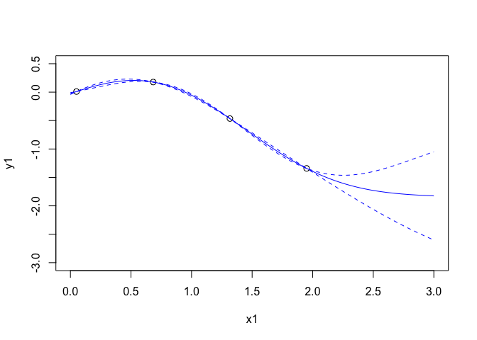
The blue lines are the mean function and prediction intervals. We can look at what has been fit here:
## [1] "Regression part:  -0.378  +  -0.394 x1"

## [1] "Half length correlation: 0.347"

## [1] "Quarter length correlation: 0.768"

## [1] "Sigma^2 =  0.378"
Now we fit an emulator using maximum likelihood (so we set the priors to be uniform, as is default in mogp)
priors <- NULL
gp1 <- mogp_emulator$GaussianProcess(inputs, targets,
                                    mean=mean_func,
                                    nugget="adaptive",
                                    inputdict=inputdict)
p1 <- mogp_emulator$fit_GP_MAP(gp1)

plot(x1,y1,xlim=c(0,3),ylim=c(-3,0.5),cex=1.1)
points(xpreds, p$theta[1] + xpreds*p$theta[2],type='l',col=4,lty=3,lwd=0.5)
tpreds <- gp$predict(xpreds,deriv = FALSE)
points(xpreds,tpreds$mean,col=4,type='l')
points(xpreds, tpreds$mean + 2*(sqrt(tpreds$unc)),col=4,type="l",lty=2)
points(xpreds, tpreds$mean - 2*(sqrt(tpreds$unc)),col=4,type="l",lty=2)
points(xpreds, p1$theta[1] + xpreds*p1$theta[2],type='l',col=2,lty=3,lwd=0.5,)
tpreds1 <- gp1$predict(xpreds,deriv = FALSE)
points(xpreds,tpreds1$mean,col=2,type='l')
points(xpreds, tpreds1$mean + 2*(sqrt(tpreds1$unc)),col=2,type="l",lty=2)
points(xpreds, tpreds1$mean - 2*(sqrt(tpreds1$unc)),col=2,type="l",lty=2)
p1$theta
## [1] 0.3373245 -0.7418168 4.6400067 -2.6284617 0.8365486
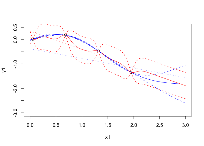
The red lines are the mean and prediction intervals for the maximum likelihood emulator. Similarly here is what has been fit.
## [1] "Regression part:  0.337  +  -0.742 x1"

## [1] "Half length correlation: 0"

## [1] "Quarter length correlation: 0"

## [1] "Sigma^2 =  0.0722"
In this case, it is clear that the maximium likelihood estimate which is on the likelihood ridge and has a large variance and low correlation everywhere. The result is an emulator with no predictive power and with a variance that is too small away from the observations.
Our prior choices are designed to push the emulator away from the likeilhood ridge, to be weakly informative (rather than uninformative) and to allow the user the flexibility to adapt some of them, particularly if they feel some variables should be active/inactive for particular outputs.
Walking through the ExeterUQ priors.
We will use the same test data as before and use a linear mean function to illustrate how we choose our priors, then describe them.
load("ConvectionModelExample.Rdata")
head(tData)
##          A_U  A_EPSILON         A_T       Noise
## 1 -0.7112332  0.5198038  0.56237588 -0.03849208
## 2 -0.2465941 -0.4163290  0.88555390 -0.02695154
## 3  0.3333848 -0.1316253  0.30027685 -0.04939970
## 4  0.4462722  0.8817862  0.78243180  0.01830642
## 5 -0.9065298 -0.3119412 -0.07690085 -0.04815524
## 6 -0.4732543  0.3305641 -0.98112145 -0.02420066
##   WAVE1_AYOTTE_24SC_zav.400.600.theta_5_6 WAVE1_AYOTTE_24SC_Ay.theta_5_6
## 1                                306.1641                     -0.3697345
## 2                                306.7235                     -0.5671676
## 3                                306.6203                     -0.4999037
## 4                                306.3918                     -0.3919627
## 5                                306.1552                     -0.3685847
## 6                                305.6225                     -0.3485485
##   WAVE1_AYOTTE_24SC_zav.400.600.WND_5_6
## 1                              13.82073
## 2                              12.25888
## 3                              11.82482
## 4                              11.94844
## 5                              14.73021
## 6                              13.17205
Kernel <- "Gaussian"
Choices <- choices.default
Choices
## $DeltaActiveMean
## [1] 0
##
## $DeltaActiveSigma
## [1] 0.125
##
## $DeltaInactiveMean
## [1] 5
##
## $DeltaInactiveSigma
## [1] 0.005
##
## $BetaRegressMean
## [1] 0
##
## $BetaRegressSigma
## [1] 10
##
## $NuggetProportion
## [1] 0.1
##
## $Nugget
## [1] "fit"
##
## $lm.tryFouriers
## [1] FALSE
##
## $lm.maxOrder
## NULL
##
## $lm.maxdf
## NULL
The default parameters we use to control mogp priors are shown above. We will go through the implications of each one and discuss what changing it does. First some preliminaries to fit a linear mean function in the parameters.
lastCand <- which(names(tData)=="Noise")
HowManyEmulators <- length(names(tData)) - lastCand
tData <- tData[,c(1:lastCand,(lastCand+1):(lastCand+HowManyEmulators))]
linPredictor <- paste(names(tData)[1:(lastCand-1)],collapse="+")
lm.list = lapply(1:HowManyEmulators, function(k) list(linModel =
    eval(parse(text = paste("lm(", paste(names(tData[lastCand+k]),
    linPredictor, sep="~"), ", data=tData)",  sep="")))))
ActiveVariableIndices <- lapply(lm.list, function(tlm) names(tData)[1:(lastCand-1)])
summary(lm.list[[1]]$linModel)
##
## Call:
## lm(formula = WAVE1_AYOTTE_24SC_zav.400.600.theta_5_6 ~ A_U +
##     A_EPSILON + A_T, data = tData)
##
## Residuals:
##      Min       1Q   Median       3Q      Max
## -0.28152 -0.15136 -0.03609  0.07924  0.84547
##
## Coefficients:
##              Estimate Std. Error  t value Pr(>|t|)
## (Intercept) 306.46468    0.04160 7366.754  < 2e-16 ***
## A_U           0.33186    0.07186    4.618 9.21e-05 ***
## A_EPSILON    -0.57679    0.07192   -8.020 1.69e-08 ***
## A_T           0.32259    0.07164    4.503 0.000125 ***
## ---
## Signif. codes:  0 '***' 0.001 '**' 0.01 '*' 0.05 '.' 0.1 ' ' 1
##
## Residual standard error: 0.2278 on 26 degrees of freedom
## Multiple R-squared:  0.8134, Adjusted R-squared:  0.7918
## F-statistic: 37.77 on 3 and 26 DF,  p-value: 1.267e-09
Now we set the required quantities to call GetPriors() so that we can
step through that code to illustrate and discuss our prior choices.
lm.emulator <- lm.list[[1]]
d <- 3
ActiveVariables <- ActiveVariableIndices[[1]]
Stepping through GetPriors()
p <- length(lm.emulator$linModel$coefficients)-1
Betas <- lapply(1:p, function(e)
                mogp_priors$NormalPrior(Choices$BetaRegressMean,
                Choices$BetaRegressSigma))
The above sets a N(BetaRegressMean, BetaRegressSigma) prior for
each of the regression coefficients but leaves the intercept as uniorm.
Our default choices are for N(0, 102)
hist(rnorm(10000,Choices$BetaRegressMean,Choices$BetaRegressSigma), breaks=100,
      main=expression(paste("Samples from the regression coefficient prior for ",
      beta,sep=" ")),xlab=expression(beta))
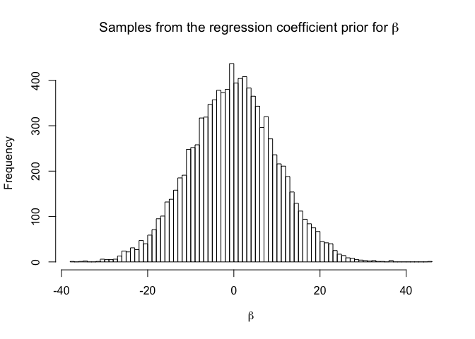
This is a relatively weak prior that should aid optimisation of MAP. The most controversial choice (from a subjective Bayesian perspective) is to allow the intercept to be uniform, but this works well in practice, particularly over many outputs. Many emulator users have output on a variety of scales and it is often impractical or undesirable for a application user to transform the output from the scale they understand to something more convenient for statistical fitting but less interpretable.
The prior on the regression coefficients could, if anything, be too tight, but this situation is rare. If a very large coefficient is suggested by the preliminary linear fit, this is a flag that something about the data makeup is unusual and that a different emulation approach might be required. For example, an input might naturally live on a log scale and need to be explored over many orders of magnitude. But if the transformation has not happened at the design stage, the data may have a dramatic non linear response to that input that requires either a more bespoke mean function with higher order polynomial terms, or a weaker prior here.
Prior variance and nugget
I am typically a fan of Gelman (2006)‘s attitude to `weakly informative’ priors for variances being half normal, as they are easier to think about and to make automatic choices for. This was our approach in our Stan release.
A price we pay for the speed brought by mogp, is that we lose the flexibility of prior modelling offered by Stan. We use the inverse gamma implementation in mogp, and attempt to set an informative prior using the information from the preliminary fitting we have.
Whilst the prior on the mean function is arguably only important in that we require sufficient flexibility, the priors on the other parameters are important as they must overcome the problem with the ridge on the Gaussian Process likelihood surface described above.
The problem is that our data are not generated from a weakly stationary Gaussian process and so, in a very many cases, solutions with means very far from the data, large variances and long correlation lengths - those on the likelihood ridge - are particularly attractive. Our priors are designed to penalise this ridge and encourage the emulator to have a variance that respects the data that we have. Ideally, the mean function explains some of the total variability in the data, so we have natural bounds on σ2 from the variability in the data and the amount of variance we would like to explain.
Though the parameters required by the mogp_emulator implementation of
the Inverse Gamma distribution are the usual shape and rate of the
distribution, we reparametrise in terms of the mode and the variance.
Once given the mode and variance, the shape parameter is a root of
V**x3 − (4V + M2)x2 + (5V − 2M2)x − (2V + M2),
and the rate parameter can be computed directly given the shape. Our
invgamMode function converts the mode and a bound on σ2
into the parameters of the inverse gamma distribution by first
considering the number of standard deviations from the mode to the given
bound to be 6 (in order to compute a variance), then solving the above
numerically to obtain the inverse gamma parameters. The subjective
choices are now the mode and bound on the variance, and we have natural
information to use given our preliminary fitting.
We take the bound to be the variance of the data scaled by
1 - Choices$NuggetProportion. This prior says that we expect
Choices$NuggetProportion of the data variance to be nugget and the
rest to be due to the GP. The argument here is that our bound accounts
for the constant mean case, but we believe some signal to be absorbed by
the mean function. The mode we set to be the variance of the residuals
of our preliminary fit. Effectively this prior allows all variances that
are consistent with the data but has vanishingly small probability for
larger variances that would then force the correlation to be very high
and place us on the likelihood ridge.
In the GetPriors() code, first the mode and bound are set, as
described above; the shape and rate are derived by calling to
invgamMode and the parameters are passed to the mogp_priors module.
  ModeSig <- var(lm.emulator$linModel$residuals)
  boundSig <- ModeSig/(1-summary(lm.emulator$linModel)$r.squared)
  SigmaParams <- invgamMode((1-Choices$NuggetProportion)*boundSig,ModeSig)
  Sigma <- mogp_priors$InvGammaPrior(SigmaParams$alpha,SigmaParams$beta)
We can see the prior for our data here, as well as calculating the prior probability of exceeding the bound.
  alphaSig <- SigmaParams$alpha
  betaSig <- SigmaParams$beta
  hist(rinvgamma(10000,alphaSig,betaSig),breaks=100,
      main = expression(paste("Samples from the prior for ", sigma^2,sep=" ")),
      xlab=expression(sigma^2))
  abline(v=ModeSig)
  abline(v=(1-Choices$NuggetProportion)*boundSig,col=2)
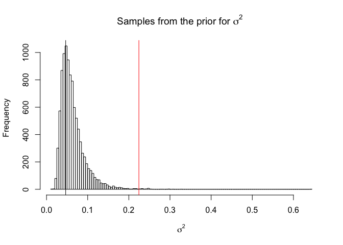
print(1-pinvgamma((1-Choices$NuggetProportion)*boundSig,alphaSig,betaSig))
## [1] 0.002377577
The nugget distribution follows similarly, setting the mode and bound to
be Choices$NuggetProportion times those used for σ2
NuggetParams <- invgamMode(Choices$NuggetProportion*boundSig ,Choices$NuggetProportion*ModeSig)
    Nugget <- mogp_priors$InvGammaPrior(NuggetParams$alpha, NuggetParams$beta)
Correlation lengths
The correlation lengths are logged throughout mogp_emulator, so we set
these logs to have a Normal prior, giving the correlation lengths a log
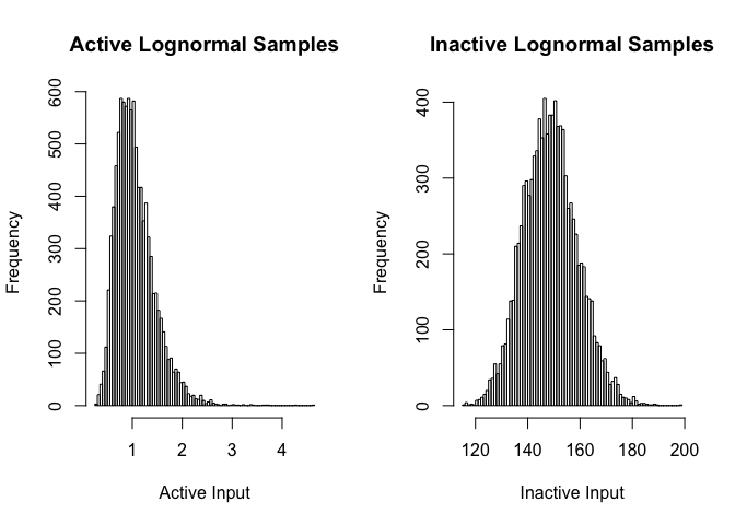
normal prior. We use the correlation lengths in our prior description to
distinguish between “active” and “inactive” inputs.
In most applications we work in, there are many more inputs than one can feasibly fit a Gaussian Process with a separable covariance to. The issue is caused by the curse of dimensionality which basically means that points one might think of as close together are actually very far away in many dimensions.
Take for example the squared exponential kernel written as a product of exponentials rather than the usual sum to illustrate the point. If each dimension contributes a high correlation (e.g. 0.9), then in 15 dimensions the overall correlation is 0.2 and in 20 it’s 0.12. But further, looking at other combinations of high correlation, you can see that correlation decays very quickly:
c(0.7,0.8,0.9)^15
## [1] 0.004747562 0.035184372 0.205891132
c(0.7,0.8,0.9)^20
## [1] 0.0007979227 0.0115292150 0.1215766546
The solution to this has been only to fit the GP part to a subset of active inputs, with the remainder being inactive (Craig et al. 1996). As we have a prior on the nugget, (and as the nugget is additive), we capture the variability from inactive inputs easily, so the main thing that needs to be achieved is to ensure inactive inputs do not kill the correlation.
We set our inactive input hyperparameters so that the correlation is very close to 1. Then, when computing a separable covariance function, those parameters do not impact on the overall covariance and so are “effectively” ignored. A different solution would be to remove them and to reshape all arrays. If all inactive correlations are 1, these solutions are equivalent.
Note that in the special case of only 1 input that is inactive, this solution really does not work. However, we assume that a modeller would not want to fit a GP to a single input and to specify that it is inactive!
par(mfrow=c(1,2))
hist(rlnorm(10000,Choices$DeltaActiveMean,sqrt(Choices$DeltaActiveSigma)), breaks=100,
      main="Active Lognormal Samples",xlab="Active Input")
hist(rlnorm(10000, Choices$DeltaInactiveMean,sqrt(Choices$DeltaInactiveSigma)), breaks=100,
      main="Inactive Lognormal Samples",xlab="Inactive Input")
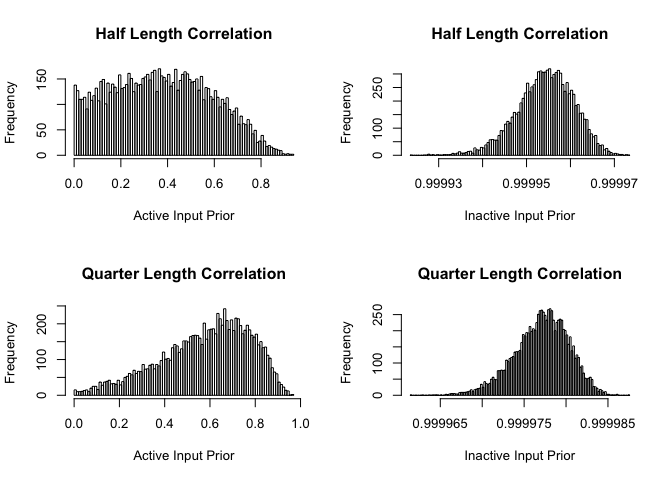
par(mfrow=c(2,2))
hist(exp(-1/rlnorm(10000, Choices$DeltaActiveMean,sqrt(Choices$DeltaActiveSigma))^2), breaks=100,
    main="Half Length Correlation", xlab="Active Input Prior")
hist(exp(-1/rlnorm(10000, Choices$DeltaInactiveMean, sqrt(Choices$DeltaInactiveSigma))^2), breaks=100,
    main="Half Length Correlation", xlab="Inactive Input Prior")
hist(exp(-.5/rlnorm(10000, Choices$DeltaActiveMean, sqrt(Choices$DeltaActiveSigma))^2),breaks=100,
    main="Quarter Length Correlation", xlab="Active Input Prior")
hist(exp(-.5/rlnorm(10000, Choices$DeltaInactiveMean, sqrt(Choices$DeltaInactiveSigma))^2),breaks=100,
    main="Quarter Length Correlation", xlab="Inactive Input Prior")