Preliminaries
First we specify the directory where mogp is installed so that the python is correctly imported. Your directory will be different from mine.
mogp_dir <- "~/Dropbox/BayesExeter/mogp_emulator"
setwd('..')
source("BuildEmulator/BuildEmulator.R")
source("HistoryMatching/HistoryMatching.R")
source("HistoryMatching/impLayoutplot.R")
We load the same data looked at in the tutorial on building emulators.
load("ConvectionModelExample.Rdata")
head(tData)
##          A_U  A_EPSILON         A_T       Noise
## 1 -0.7112332  0.5198038  0.56237588 -0.03849208
## 2 -0.2465941 -0.4163290  0.88555390 -0.02695154
## 3  0.3333848 -0.1316253  0.30027685 -0.04939970
## 4  0.4462722  0.8817862  0.78243180  0.01830642
## 5 -0.9065298 -0.3119412 -0.07690085 -0.04815524
## 6 -0.4732543  0.3305641 -0.98112145 -0.02420066
##   WAVE1_AYOTTE_24SC_zav.400.600.theta_5_6 WAVE1_AYOTTE_24SC_Ay.theta_5_6
## 1                                306.1641                     -0.3697345
## 2                                306.7235                     -0.5671676
## 3                                306.6203                     -0.4999037
## 4                                306.3918                     -0.3919627
## 5                                306.1552                     -0.3685847
## 6                                305.6225                     -0.3485485
##   WAVE1_AYOTTE_24SC_zav.400.600.WND_5_6
## 1                              13.82073
## 2                              12.25888
## 3                              11.82482
## 4                              11.94844
## 5                              14.73021
## 6                              13.17205
Build an emulator.
TestEm <- BuildNewEmulators(tData, HowManyEmulators = 3, meanFun = "fitted")
## [1] "Max reduction is 0.141510566268957 using A_EPSILON"
## [1] "Max reduction is 0.0719279431890675 using A_U"
## [1] "Max reduction is 0.0593934956606317 using A_T"
## [1] "Max reduction is 0.0841015596079704 using A_EPSILON"
## [1] "Max reduction is 0.0215815680504046 using A_EPSILON"
## [1] "Max reduction is 0.0221974794878812 using A_EPSILON"
## [1] "Noise fitted, stopping algorithm"
##
## Call:
## lm(formula = WAVE1_AYOTTE_24SC_zav.400.600.theta_5_6 ~ A_EPSILON +
##     I(A_EPSILON^2) + I(A_EPSILON^3) + I(A_EPSILON^4) + A_U +
##     A_T + I(A_U * A_EPSILON) + I(A_T * A_EPSILON) + I(A_T * A_U),
##     data = tData)
##
## Residuals:
##      Min       1Q   Median       3Q      Max
## -0.15059 -0.06624  0.01615  0.05931  0.15216
##
## Coefficients:
##                     Estimate Std. Error  t value Pr(>|t|)
## (Intercept)        306.35982    0.03461 8852.437  < 2e-16 ***
## A_EPSILON           -0.31275    0.08180   -3.824  0.00106 **
## I(A_EPSILON^2)      -0.19500    0.21788   -0.895  0.38145
## I(A_EPSILON^3)      -0.43915    0.12490   -3.516  0.00217 **
## I(A_EPSILON^4)       0.83401    0.24582    3.393  0.00289 **
## A_U                  0.30423    0.03234    9.409 8.73e-09 ***
## A_T                  0.33990    0.03172   10.715 9.78e-10 ***
## I(A_U * A_EPSILON)  -0.08042    0.05404   -1.488  0.15233
## I(A_T * A_EPSILON)  -0.08069    0.06159   -1.310  0.20500
## I(A_T * A_U)        -0.03824    0.06560   -0.583  0.56648
## ---
## Signif. codes:  0 '***' 0.001 '**' 0.01 '*' 0.05 '.' 0.1 ' ' 1
##
## Residual standard error: 0.09867 on 20 degrees of freedom
## Multiple R-squared:  0.9731, Adjusted R-squared:  0.961
## F-statistic: 80.31 on 9 and 20 DF,  p-value: 1.004e-13
##
##
## Call:
## lm(formula = WAVE1_AYOTTE_24SC_zav.400.600.theta_5_6 ~ A_EPSILON +
##     I(A_EPSILON^2) + I(A_EPSILON^3) + I(A_EPSILON^4) + A_U +
##     A_T + I(A_U * A_EPSILON) + I(A_T * A_EPSILON) + I(A_T * A_U),
##     data = tData)
##
## Residuals:
##      Min       1Q   Median       3Q      Max
## -0.15059 -0.06624  0.01615  0.05931  0.15216
##
## Coefficients:
##                     Estimate Std. Error  t value Pr(>|t|)
## (Intercept)        306.35982    0.03461 8852.437  < 2e-16 ***
## A_EPSILON           -0.31275    0.08180   -3.824  0.00106 **
## I(A_EPSILON^2)      -0.19500    0.21788   -0.895  0.38145
## I(A_EPSILON^3)      -0.43915    0.12490   -3.516  0.00217 **
## I(A_EPSILON^4)       0.83401    0.24582    3.393  0.00289 **
## A_U                  0.30423    0.03234    9.409 8.73e-09 ***
## A_T                  0.33990    0.03172   10.715 9.78e-10 ***
## I(A_U * A_EPSILON)  -0.08042    0.05404   -1.488  0.15233
## I(A_T * A_EPSILON)  -0.08069    0.06159   -1.310  0.20500
## I(A_T * A_U)        -0.03824    0.06560   -0.583  0.56648
## ---
## Signif. codes:  0 '***' 0.001 '**' 0.01 '*' 0.05 '.' 0.1 ' ' 1
##
## Residual standard error: 0.09867 on 20 degrees of freedom
## Multiple R-squared:  0.9731, Adjusted R-squared:  0.961
## F-statistic: 80.31 on 9 and 20 DF,  p-value: 1.004e-13
##
## [1] "1 I(A_T * A_U)"
## [1] "2 I(A_T * A_EPSILON)"
## [1] "3 I(A_U * A_EPSILON)"
## [1] "4 I(A_EPSILON^4)"
## [1] "5 I(A_EPSILON^3)"
##
## Call:
## lm(formula = WAVE1_AYOTTE_24SC_zav.400.600.theta_5_6 ~ A_EPSILON +
##     I(A_EPSILON^2) + A_U + A_T, data = tData)
##
## Residuals:
##      Min       1Q   Median       3Q      Max
## -0.31141 -0.07230  0.00132  0.06857  0.49418
##
## Coefficients:
##                 Estimate Std. Error  t value Pr(>|t|)
## (Intercept)    306.28286    0.04193 7304.864  < 2e-16 ***
## A_EPSILON       -0.57626    0.04796  -12.015 7.00e-12 ***
## I(A_EPSILON^2)   0.53877    0.09315    5.784 4.98e-06 ***
## A_U              0.32558    0.04794    6.792 4.06e-07 ***
## A_T              0.34208    0.04790    7.142 1.74e-07 ***
## ---
## Signif. codes:  0 '***' 0.001 '**' 0.01 '*' 0.05 '.' 0.1 ' ' 1
##
## Residual standard error: 0.152 on 25 degrees of freedom
## Multiple R-squared:  0.9202, Adjusted R-squared:  0.9074
## F-statistic: 72.06 on 4 and 25 DF,  p-value: 2.36e-13
##
## [1] "Max reduction is 0.0516838339369975 using A_EPSILON"
## [1] "Max reduction is 0.0181512292708917 using A_T"
## [1] "Max reduction is 0.00908627733663028 using A_U"
## [1] "Noise fitted, stopping algorithm"
##
## Call:
## lm(formula = WAVE1_AYOTTE_24SC_Ay.theta_5_6 ~ A_EPSILON + A_T +
##     A_U + I(A_T * A_EPSILON) + I(A_U * A_EPSILON) + I(A_U * A_T),
##     data = tData)
##
## Residuals:
##       Min        1Q    Median        3Q       Max
## -0.122972 -0.017118  0.003162  0.026879  0.108563
##
## Coefficients:
##                     Estimate Std. Error t value Pr(>|t|)
## (Intercept)        -0.466705   0.009108 -51.243  < 2e-16 ***
## A_EPSILON           0.173565   0.015924  10.900 1.47e-10 ***
## A_T                -0.078502   0.015793  -4.971 5.01e-05 ***
## A_U                -0.050460   0.015915  -3.171  0.00427 **
## I(A_T * A_EPSILON)  0.066547   0.030606   2.174  0.04022 *
## I(A_U * A_EPSILON) -0.025424   0.025766  -0.987  0.33405
## I(A_U * A_T)       -0.035683   0.031953  -1.117  0.27564
## ---
## Signif. codes:  0 '***' 0.001 '**' 0.01 '*' 0.05 '.' 0.1 ' ' 1
##
## Residual standard error: 0.0496 on 23 degrees of freedom
## Multiple R-squared:  0.8819, Adjusted R-squared:  0.8511
## F-statistic: 28.62 on 6 and 23 DF,  p-value: 1.439e-09
##
##
## Call:
## lm(formula = WAVE1_AYOTTE_24SC_Ay.theta_5_6 ~ A_EPSILON + A_T +
##     A_U + I(A_T * A_EPSILON) + I(A_U * A_EPSILON) + I(A_U * A_T),
##     data = tData)
##
## Residuals:
##       Min        1Q    Median        3Q       Max
## -0.122972 -0.017118  0.003162  0.026879  0.108563
##
## Coefficients:
##                     Estimate Std. Error t value Pr(>|t|)
## (Intercept)        -0.466705   0.009108 -51.243  < 2e-16 ***
## A_EPSILON           0.173565   0.015924  10.900 1.47e-10 ***
## A_T                -0.078502   0.015793  -4.971 5.01e-05 ***
## A_U                -0.050460   0.015915  -3.171  0.00427 **
## I(A_T * A_EPSILON)  0.066547   0.030606   2.174  0.04022 *
## I(A_U * A_EPSILON) -0.025424   0.025766  -0.987  0.33405
## I(A_U * A_T)       -0.035683   0.031953  -1.117  0.27564
## ---
## Signif. codes:  0 '***' 0.001 '**' 0.01 '*' 0.05 '.' 0.1 ' ' 1
##
## Residual standard error: 0.0496 on 23 degrees of freedom
## Multiple R-squared:  0.8819, Adjusted R-squared:  0.8511
## F-statistic: 28.62 on 6 and 23 DF,  p-value: 1.439e-09
##
## [1] "1 I(A_U * A_EPSILON)"
## [1] "2 I(A_U * A_T)"
##
## Call:
## lm(formula = WAVE1_AYOTTE_24SC_Ay.theta_5_6 ~ A_EPSILON + A_T +
##     A_U + I(A_T * A_EPSILON), data = tData)
##
## Residuals:
##       Min        1Q    Median        3Q       Max
## -0.125503 -0.019057  0.002386  0.026174  0.097011
##
## Coefficients:
##                     Estimate Std. Error t value Pr(>|t|)
## (Intercept)        -0.466250   0.009099 -51.240  < 2e-16 ***
## A_EPSILON           0.175425   0.015790  11.110 3.68e-11 ***
## A_T                -0.076189   0.015710  -4.850 5.50e-05 ***
## A_U                -0.052910   0.015894  -3.329   0.0027 **
## I(A_T * A_EPSILON)  0.064706   0.030065   2.152   0.0412 *
## ---
## Signif. codes:  0 '***' 0.001 '**' 0.01 '*' 0.05 '.' 0.1 ' ' 1
##
## Residual standard error: 0.04981 on 25 degrees of freedom
## Multiple R-squared:  0.8705, Adjusted R-squared:  0.8498
## F-statistic: 42.01 on 4 and 25 DF,  p-value: 9.526e-11
##
## [1] "Max reduction is 0.482408369617749 using A_U"
## [1] "Max reduction is 0.218319375740367 using A_U"
## [1] "Max reduction is 0.125730158685294 using A_EPSILON"
## [1] "Max reduction is 0.0997702118329568 using A_U"
## [1] "Max reduction is 0.0271958533098509 using A_U"
## [1] "Max reduction is 0.0170111124043587 using A_U"
## [1] "Max reduction is 0.00102285247477041 using A_EPSILON"
## [1] "Max reduction is 0.0269160398536438 using Three Way Interactions with A_EPSILON"
## [1] "Max reduction is 0.017685867543131 using A_T"
## [1] "No further terms permitted with the given degrees of freedom"
##
## Call:
## lm(formula = WAVE1_AYOTTE_24SC_zav.400.600.WND_5_6 ~ A_U + I(A_U^2) +
##     I(A_U^3) + I(A_U^4) + I(A_U^5) + A_EPSILON + I(A_EPSILON^2) +
##     A_T + I(A_EPSILON * A_U) + I(A_T * A_U) + I(A_T * A_EPSILON) +
##     I(A_EPSILON * A_EPSILON * A_U) + I(A_EPSILON * A_T * A_U) +
##     I(A_EPSILON * A_T * A_EPSILON), data = tData)
##
## Residuals:
##       Min        1Q    Median        3Q       Max
## -0.096819 -0.014154  0.003559  0.029044  0.061739
##
## Coefficients:
##                                Estimate Std. Error t value Pr(>|t|)
## (Intercept)                    12.14491    0.02127 570.984  < 2e-16 ***
## A_U                            -1.19660    0.07737 -15.466 1.26e-10 ***
## I(A_U^2)                        0.49853    0.11485   4.341 0.000582 ***
## I(A_U^3)                        0.04079    0.29706   0.137 0.892609
## I(A_U^4)                        1.02544    0.12295   8.340 5.14e-07 ***
## I(A_U^5)                       -1.08677    0.24586  -4.420 0.000496 ***
## A_EPSILON                       0.31898    0.01865  17.100 3.01e-11 ***
## I(A_EPSILON^2)                 -0.13457    0.03630  -3.707 0.002109 **
## A_T                            -0.02568    0.02879  -0.892 0.386454
## I(A_EPSILON * A_U)             -0.38773    0.03026 -12.814 1.75e-09 ***
## I(A_T * A_U)                    0.11796    0.03987   2.959 0.009760 **
## I(A_T * A_EPSILON)             -0.04880    0.03605  -1.354 0.195903
## I(A_EPSILON * A_EPSILON * A_U)  0.38672    0.06230   6.208 1.68e-05 ***
## I(A_EPSILON * A_T * A_U)        0.11912    0.09194   1.296 0.214675
## I(A_EPSILON * A_T * A_EPSILON)  0.06014    0.08302   0.724 0.479946
## ---
## Signif. codes:  0 '***' 0.001 '**' 0.01 '*' 0.05 '.' 0.1 ' ' 1
##
## Residual standard error: 0.05397 on 15 degrees of freedom
## Multiple R-squared:  0.9987, Adjusted R-squared:  0.9975
## F-statistic:   813 on 14 and 15 DF,  p-value: < 2.2e-16
##
## [1] "1 I(A_EPSILON * A_T * A_EPSILON)"
## [1] "2 I(A_T * A_EPSILON)"
##
## Call:
## lm(formula = WAVE1_AYOTTE_24SC_zav.400.600.WND_5_6 ~ A_U + I(A_U^2) +
##     I(A_U^3) + I(A_U^4) + I(A_U^5) + A_EPSILON + I(A_EPSILON^2) +
##     A_T + I(A_EPSILON * A_U) + I(A_T * A_U) + I(A_EPSILON * A_EPSILON *
##     A_U) + I(A_EPSILON * A_T * A_U), data = tData)
##
## Residuals:
##       Min        1Q    Median        3Q       Max
## -0.100346 -0.022345  0.004853  0.026981  0.085676
##
## Coefficients:
##                                Estimate Std. Error t value Pr(>|t|)
## (Intercept)                    12.14806    0.02138 568.288  < 2e-16 ***
## A_U                            -1.20582    0.07347 -16.413 7.36e-12 ***
## I(A_U^2)                        0.48268    0.11484   4.203 0.000598 ***
## I(A_U^3)                        0.09328    0.28155   0.331 0.744448
## I(A_U^4)                        1.03694    0.12313   8.422 1.80e-07 ***
## I(A_U^5)                       -1.13282    0.23941  -4.732 0.000193 ***
## A_EPSILON                       0.32289    0.01861  17.351 3.01e-12 ***
## I(A_EPSILON^2)                 -0.14090    0.03560  -3.958 0.001015 **
## A_T                            -0.01237    0.01781  -0.694 0.496884
## I(A_EPSILON * A_U)             -0.39676    0.02984 -13.295 2.07e-10 ***
## I(A_T * A_U)                    0.13192    0.03907   3.376 0.003589 **
## I(A_EPSILON * A_EPSILON * A_U)  0.39776    0.05808   6.848 2.83e-06 ***
## I(A_EPSILON * A_T * A_U)        0.10485    0.08882   1.180 0.254096
## ---
## Signif. codes:  0 '***' 0.001 '**' 0.01 '*' 0.05 '.' 0.1 ' ' 1
##
## Residual standard error: 0.05457 on 17 degrees of freedom
## Multiple R-squared:  0.9985, Adjusted R-squared:  0.9974
## F-statistic: 927.6 on 12 and 17 DF,  p-value: < 2.2e-16
##
## [1] "1 I(A_EPSILON * A_T * A_U)"
## [1] "2 I(A_EPSILON^2)"
## [1] "3 I(A_T * A_U)"

## Warning in all(lapply(ThreeWayInters, function(e) (all(e[variableNum, ] < :
## coercing argument of type 'list' to logical

## [1] "4 A_T"
## [1] "5 I(A_EPSILON * A_EPSILON * A_U)"
## [1] "6 I(A_U^5)"
## [1] "7 I(A_U^4)"
## [1] "8 I(A_EPSILON * A_U)"
##
## Call:
## lm(formula = WAVE1_AYOTTE_24SC_zav.400.600.WND_5_6 ~ A_U + I(A_U^2) +
##     I(A_U^3) + A_EPSILON, data = tData)
##
## Residuals:
##      Min       1Q   Median       3Q      Max
## -0.70366 -0.10215  0.00988  0.08980  0.42528
##
## Coefficients:
##             Estimate Std. Error t value Pr(>|t|)
## (Intercept) 12.00348    0.06088 197.177  < 2e-16 ***
## A_U         -0.75201    0.16969  -4.432 0.000163 ***
## I(A_U^2)     1.44290    0.13363  10.798 6.66e-11 ***
## I(A_U^3)    -1.24241    0.25153  -4.939 4.36e-05 ***
## A_EPSILON    0.32197    0.07089   4.542 0.000122 ***
## ---
## Signif. codes:  0 '***' 0.001 '**' 0.01 '*' 0.05 '.' 0.1 ' ' 1
##
## Residual standard error: 0.2234 on 25 degrees of freedom
## Multiple R-squared:  0.9624, Adjusted R-squared:  0.9564
## F-statistic:   160 on 4 and 25 DF,  p-value: < 2.2e-16
History matching example
The history matching codes we have included target multiple
implausibility, plotting, and analyses over many waves. They are also
generalised for basis emulation which will be added to this repository
soon. We do not yet have a simple function historyMatching() that
implements the steps below with an sequence of waves of mogp emulators,
so we take you through a step by step use of our history matching codes
for a single wave below. Something more general that wraps the steps
below for multiple waves will be written in a future update.
The discrepancy variances for each output, the observations and the error on the observations are required for history matching.
tDisc <- c(0.15,0.05,0.1)
tObs <- c(306, 0.45, 12.4)
tObsErr <- c(0.15,0.05,0.1)
We generate a random sample in the parameter space and calculate the implausibility across all of the outputs simultaneously. We have included a time stamp to show how fast this is for 1 million samples thanks to mogp.
sample_size <- 1000000
nparam <- length(names(TestEm$fitting.elements$Design))
Xp <- as.data.frame(2*randomLHS(sample_size, nparam)-1)
names(Xp) <- names(TestEm$fitting.elements$Design)
system.time(Timps <- ImplausibilityMOGP(NewData=Xp, Emulator=TestEm, Discrepancy=tDisc,
                Obs=tObs, ObsErr=tObsErr))
##    user  system elapsed
##   8.862   2.860   3.560
We collect the inputs and the implausibilities for each output into a matrix
ImpData_wave1 = cbind(Xp, Timps)
and define some of the elements required for history matching. We need the number of outputs that can exceed the implausibility cutoff, the cutoff itself (often 3 by default in the literature), and the standard parameters of the model mapped to [-1,1].
VarNames <- names(Xp)
valmax = 0 #how many outputs can be above the implausibility cut off?
cutoff_vec <- 3 #the implausibility cut off
param.defaults.norm=rep(0,nparam) #the default parameters of the model (on [-1,1])
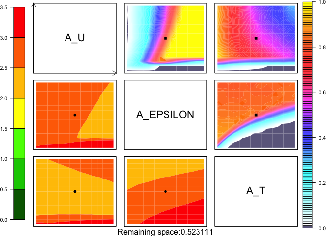
The sampled implausibilities are then used to find NROY space and to create matrices for plotting 2D projections of parameter space.
ImpListM1 = CreateImpList(whichVars = 1:nparam, VarNames=VarNames, ImpData=ImpData_wave1,
                            nEms=TestEm$mogp$n_emulators, whichMax=valmax+1)
NROY1 <- which(rowSums(Timps <= cutoff_vec[1]) >= TestEm$mogp$n_emulators -valmax)
length(NROY1)/dim(Xp)[1]
## [1] 0.523111
NROY density plots
imp.layoutm11(ImpListM1, VarNames, VariableDensity=FALSE, newPDF=FALSE,
                the.title=paste("InputSpace_wave",WAVEN,".pdf",sep=""),
                newPNG=FALSE, newJPEG=FALSE, newEPS=FALSE,
                Points=matrix(param.defaults.norm,ncol=nparam))
mtext(paste("Remaining space:",length(NROY1)/dim(Xp)[1],sep=""), side=1)